Example of Water Fall Charts - 2

I wrote Water Fall Chart example yesterday.

It became very long post.

But actually here is much simpler way to create a Water Fall Charts.

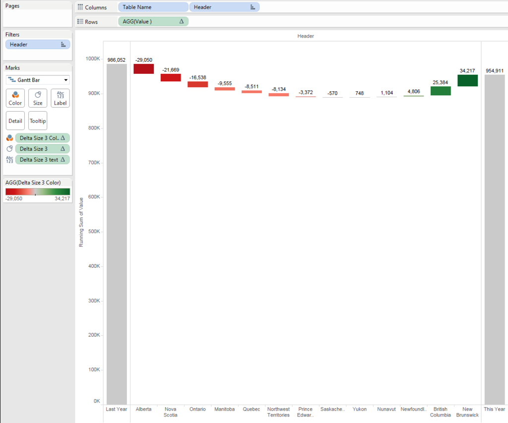
Using this way, we can create a chart on one worksheet, no need to create dashboard to combine three charts.

This is the huge benefit.

However, we need to use "Union" to triple the data, which is sometimes not available because 

- Union is only available version 9.3 or newer

- Some data connection types does not allow to us Union

- Union might cause the performance issue because of tripled data

In other words, as long as the above conditions ares not concerns, you can enjoy much simpler solution.

OK, let's start with Union.

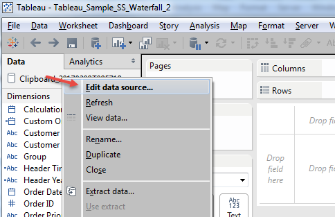
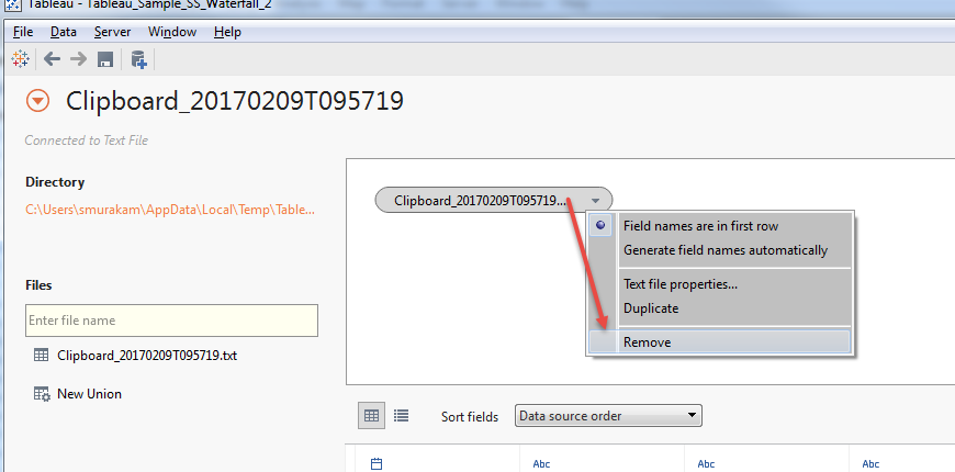
Now we have new field "Table Name".

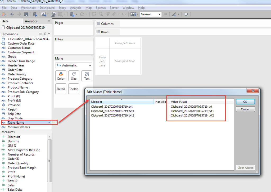
Then we can use "Table Name" as additional dimensions which make us easy to control both header and measures.

Let me explain.

The initial difficulty of water fall chart was how to conbine "Last Year" and "This Year" as bucket sum, and "Delta" as break-down to Province.

With having additional dimension, we can control this.

[Header 2]

if [Table Name]="Clipboard_20170209T095719.txt" then "Last Year"
elseif [Table Name]="Clipboard_20170209T095719.txt1" then "This Year"
else [Province] end

Talking about measusres, one important consideration is needed with this approach.

Because we tripled all the ata with Union, to get corect numbers, we always take care to avoid data duplication.

In case of LOD, we need to specify the [Table Name].

[Sales Last year]
{fixed [Table Name]:sum(if [Header Time Range] ="Last Year 3 months" then [Sales] else 0 end)}

[Sales This year]
{fixed[Table Name]:sum(if [Header Time Range] ="Curent 3 months" then [Sales] else 0 end)}

[Sales Delta]
sum(if [Header Time Range] ="Curent 3 months" then [Sales] else 0 end)

-
sum(if [Header Time Range] ="Last Year 3 months" then [Sales] else 0 end)

// We aggregates the measure and need to add "attr" on [Table Name]

 [Delta Height]

 if attr([Table Name])="Clipboard_20170209T095719.txt"
then min([Sales Last year])
elseif attr([Table Name])="Clipboard_20170209T095719.txt1"
then min([Sales This year])
else [Sales Delta] end

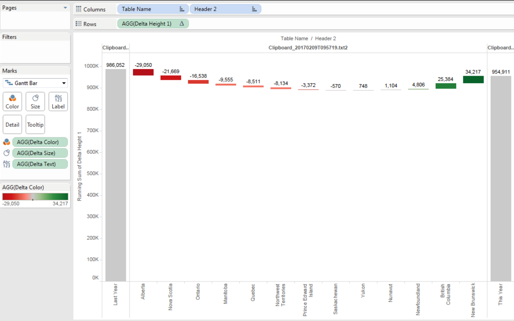
 You can get this height of Gantt.

Because the delta should be cumulated and sorted, add table calculation of "running_sum" and sort acsending.

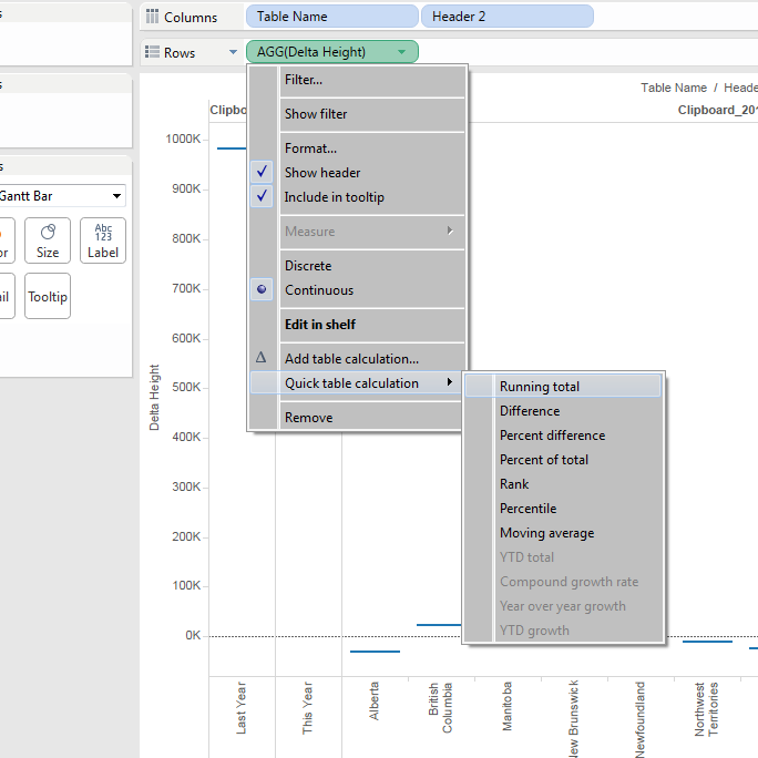
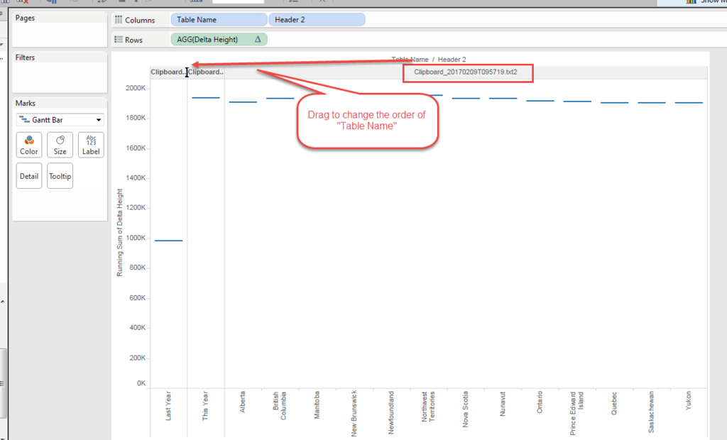
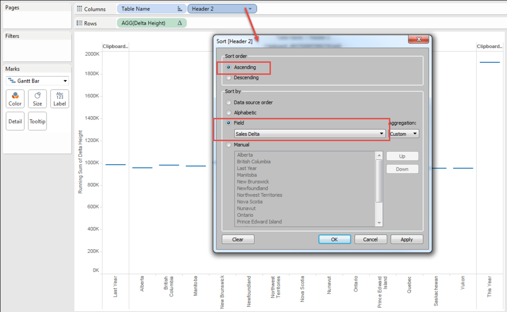
You can see the height with "running_sum" does not work on "This year", because this year is already the result of "Last year" + "Delta".

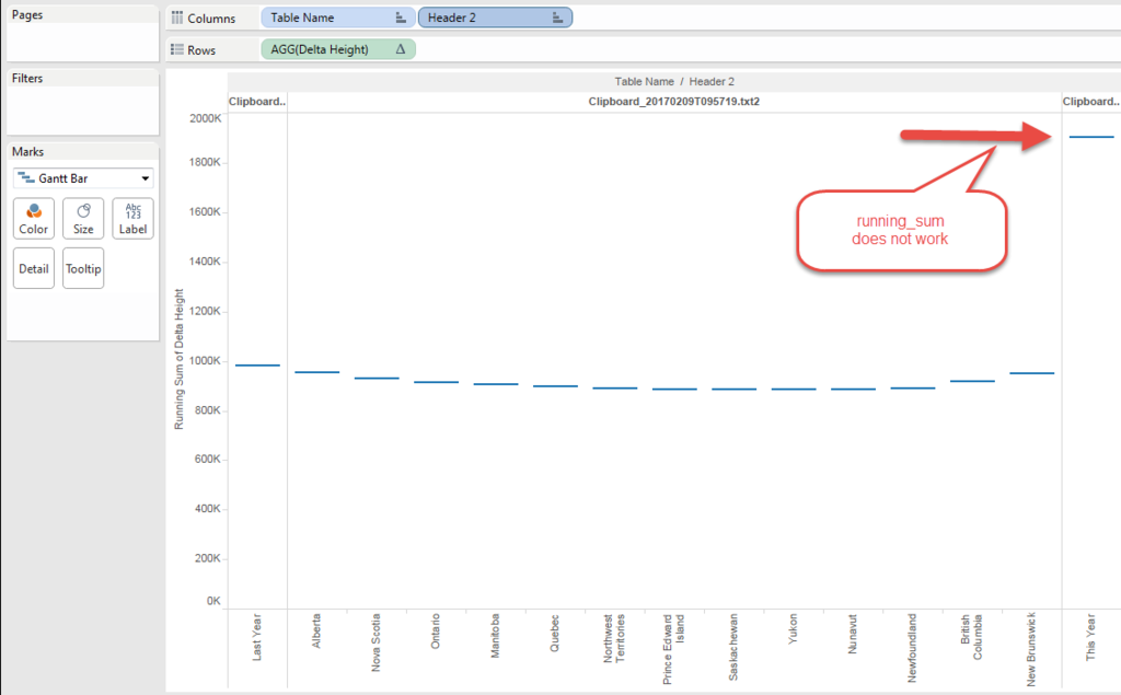
So I need to chage the formula little bit.

[Delta Height 1]

if attr([Table Name])="Clipboard_20170209T095719.txt"
then min([Sales Last year])

elseif attr([Table Name])="Clipboard_20170209T095719.txt1"
then 0
else [Sales Delta] end

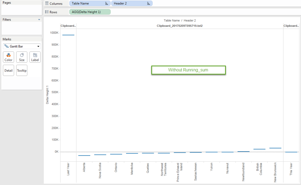
Height is done!!

Then try put "Size".

Again, the sie should be negative becasue that color need to connect the gap between the current height and previous( next left ) height.

Plus, for "Last Year" and "This Year", whole the "Height" should be the "Size" to fill to the bottom of the chart.

[Delta Size]

if attr([Table Name])="Clipboard_20170209T095719.txt"
then - min([Sales Last year])
elseif attr([Table Name])="Clipboard_20170209T095719.txt1"
then - min([Sales This year])
else -([Sales Delta])
end

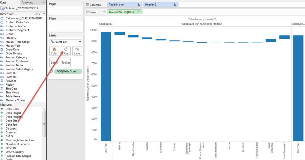
We got it!!

Then Text.

Because the "Size" is negative, to put text label we need to add field for text.

Simply

[Delta Text]

- [Delta Size]

Then put color.

When we put [Delta Text] to color, the delta color is not recognizable becasue the scale is too much different from "Last Year" and "This Year".

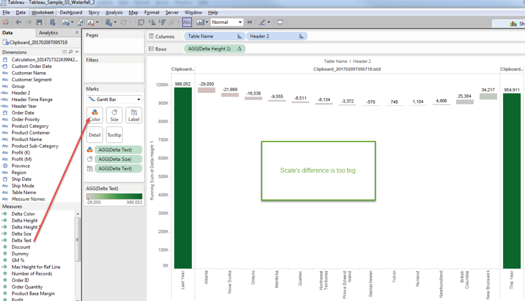
So we also need to create another calculated field to show "Color".

[Delta Color]
if attr([Table Name])="Clipboard_20170209T095719.txt2" then [Delta Text]
else 0 end

We can force the "Last Year" and "This Year" value as 0 only show the value on "Delta", by specifying the [Table Name].

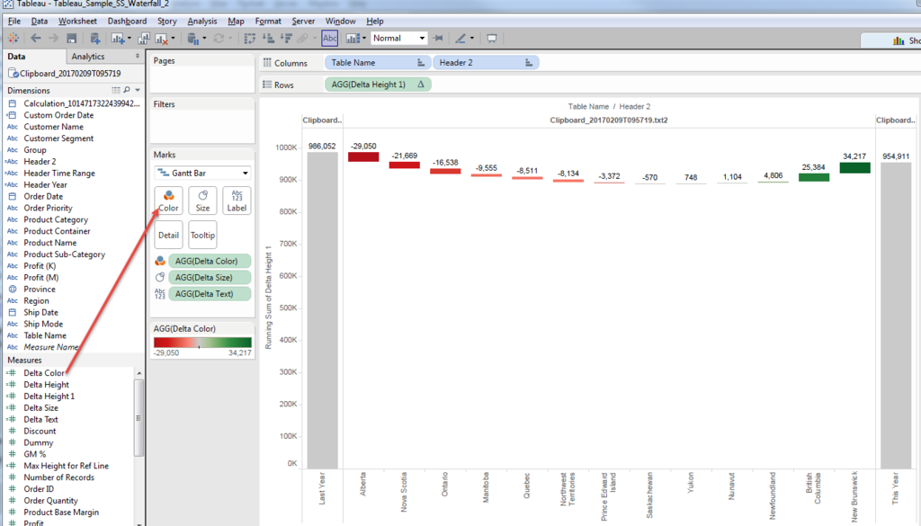
Much better.

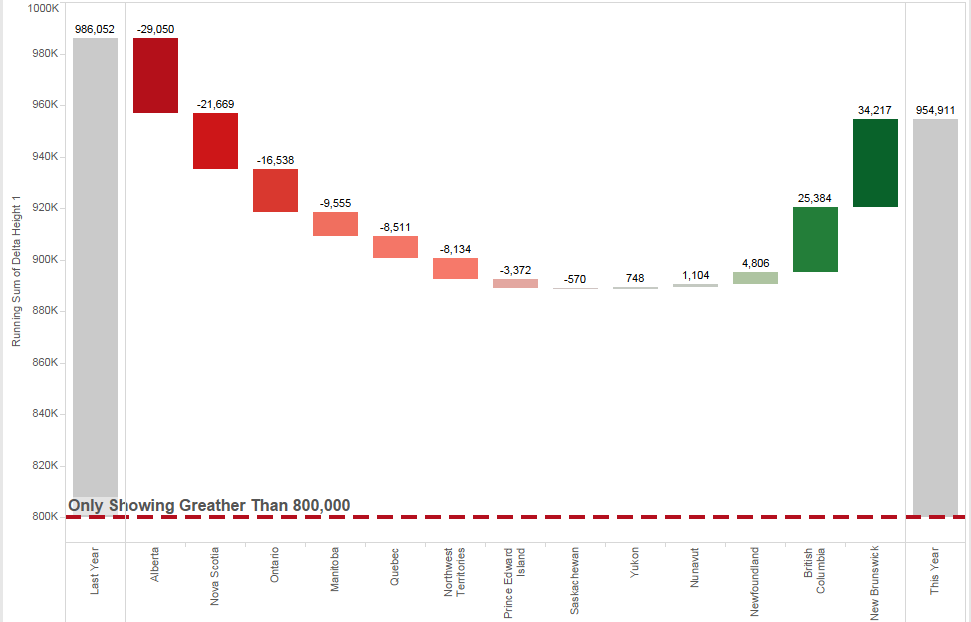
Then the merit of this approach is very flexible Y-axis modification.

For example, when we'd like to highlight the "Delta" scale.

I know not starting from "Zero" on Bar graph is sometimes not good way, though,

I understand the request is also reasonable.

In case of Gannt Chart, "excluding Zero" does not change the Y-axis range.

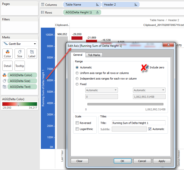
Because the size of both left/right end reaches to the bottom.

Anyways,we want to specify the minimum line.

We want to use 90% o the minium value with round.

[Minimum]

round(window_min(running_sum([Delta Height 1]))*0.9,-4)

Then we can shorten the size of Gantt with this line.

[Delta Size 2]

if attr([Table Name])="Clipboard_20170209T095719.txt"
then - (min([Sales Last year])-[Minimum])
elseif attr([Table Name])="Clipboard_20170209T095719.txt1"
then - (min([Sales This year])-[Minimum])
else -([Sales Delta])
end

And add [Minimum] to reference line.

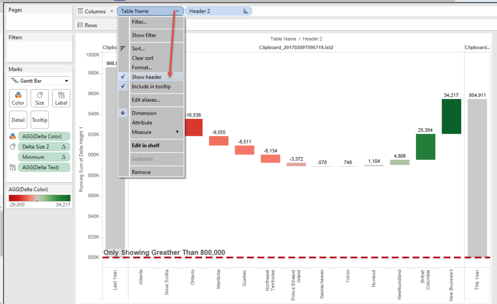
And change the format a little bit.

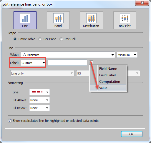
Only Showing Greater Than <Value>

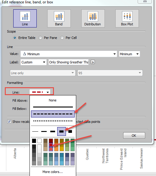
Hide Header 

And finally got the chart like this.

Tableau Public

This becomes another long post....

Anyways,  

Enjoy Tableau !!