Example of Water Fall Charts -1
Temprture is getting wamer and spring is aruond the corner!
I got couple of questions regarding Water Fall Chart.
So I post the one exapmle here.
Of course there are multiple methods to create the charts and this is not always the simplest way.
Goal is....
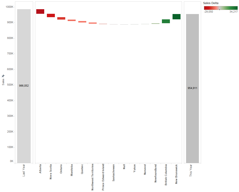
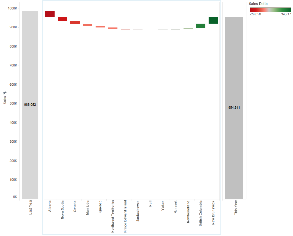
Compare This year's "The latest full three month" and "Last year's same period"
For example, today is Feb 8th , so we need to compare 2016/11~2017/02 with 2015/11~2016/02.
And we also need to show Delta break down.
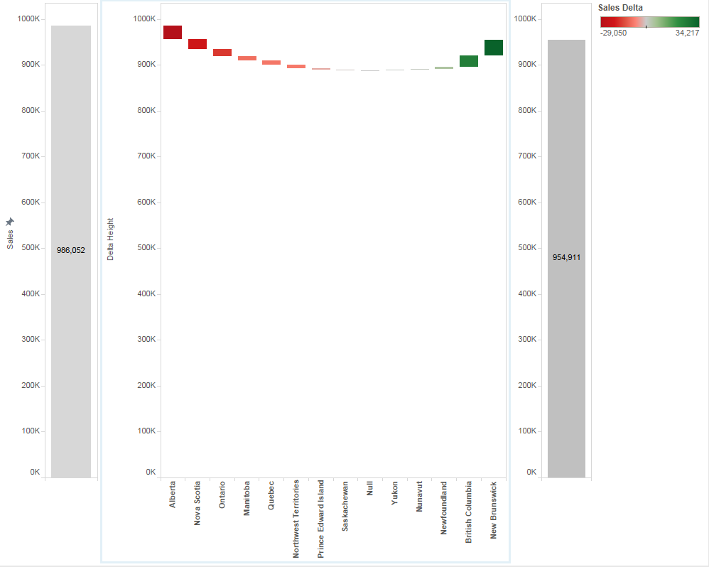
The Final Chart image is like below.
Starting from Calculated Field.
[Header Time Range]
if [Custom Order Date] <= datetrunc('month',today())-1
and
[Custom Order Date] >=dateadd('month',-3,(datetrunc('month',today())))
then "Curent 3 months"
elseif [Custom Order Date] <= dateadd('month',-12,datetrunc('month',today())-1))
and
[Custom Order Date] >=dateadd('month',-15,(datetrunc('month',today())) )
then "Last Year 3 months"
end
Datetrunc brings the first date of month and "datetrunc('month',[date])-1 " brings the last date of last month.
"dateadd('month',[date])" is shifting the date by month.
One note here is that to shift one year, we'd better use "12 months" than "1 year" to avoid an error on "2/29 of Leap Year".
It correctly select the range.
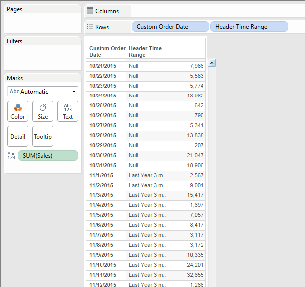
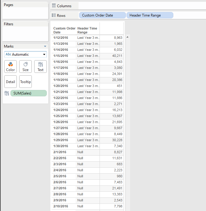
We will create three worksheets and combine on Dashboard.
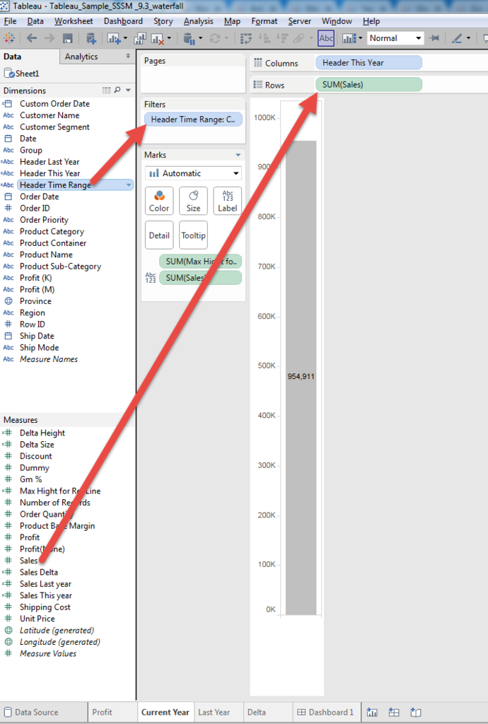
1. Current year Worksheet (Bar Chart)
Put "Sales" on Rows and Put "Header Tiemn Range" on Filter.
Then select "Curent 3 months" on filter.
2. Last year Worksheet (Bar Chart)
Put "Sales" on Rows and Put "Header Tiemn Range" on Filter.
Then select "Last Year 3 months" on filter.
3. Create Delta Worksheet (Gantt Chart)
First, calculate the delta between this year and lat year.
[Sales Delta]
sum(if [Header Time Range] ="Curent 3 months" then [Sales] else 0 end)
-
sum(if [Header Time Range] ="Last Year 3 months" then [Sales] else 0 end)
Gantt is consist of "Heighet" and "Size".
Height:
[Sales Last year]
{fixed:sum(if [Header Time Range] ="Last Year 3 months" then [Sales] else 0 end)}
[Delta Height]
attr([Sales Last year]) + running_sum([Sales Delta])
Adding each "Provinve" (in this case) delta on Last year's sales.
Using LOD brings Last year's Sales and using running_sum brings sequential height for respective "Province".
[Delta Size]
-[Sales Delta]
Size should be "Negative" in this case, because the hight is "Last year" + "Delta".
And the colored part should bridge between Current height and previous height. (Next left)
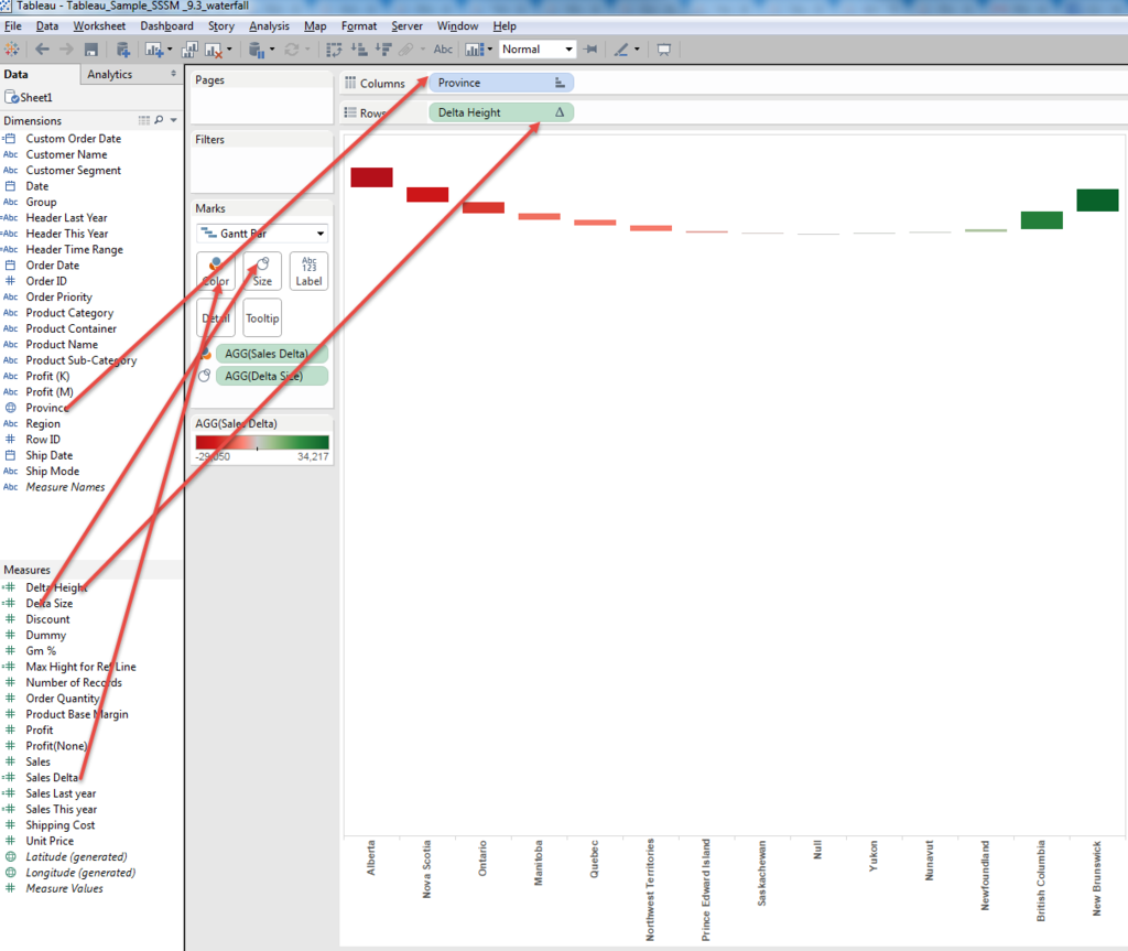
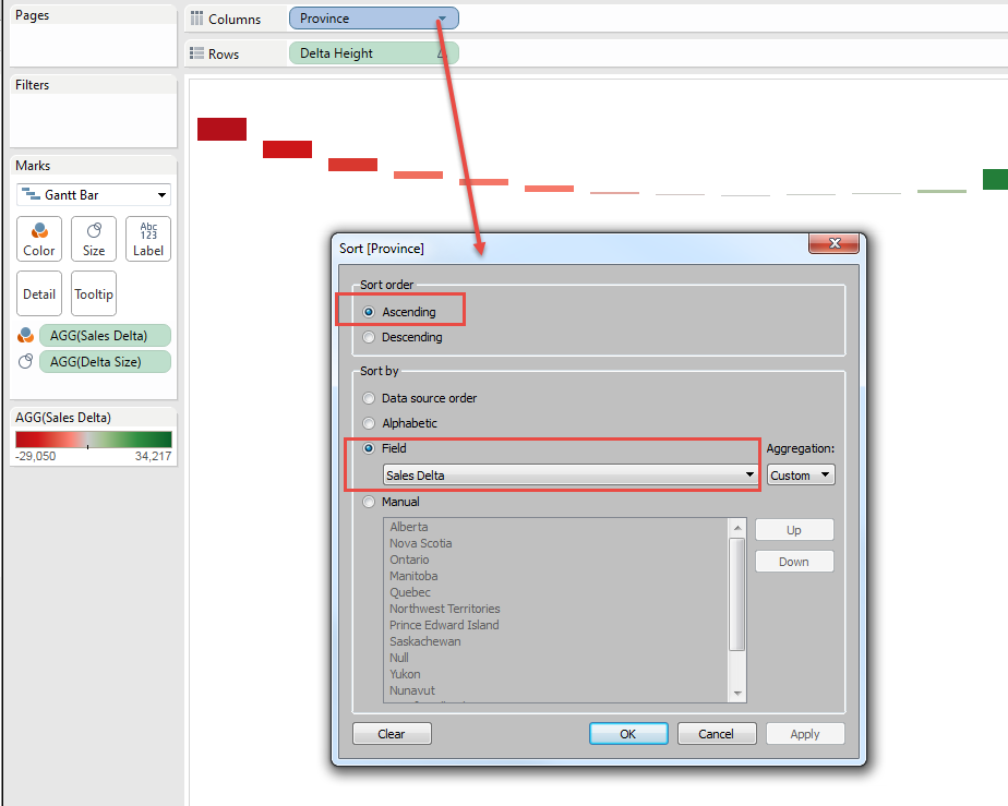
Sort Province with "Delta" Ascending.
The reason to use "Ascending", not "Descending" is to keep the total height of Graph shorter to show maximum Range.
If we take opposite way, the "Hill" is made and grapgh range(height) becomes unneccessarily tall.
Now let's try to put three worsheets on dashboard.
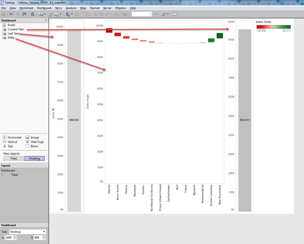
We see couple of problems.
1. Height is not aligned beteween Current and other tow.
2. Y-axis Zero line is not alighned between Delta and other two.
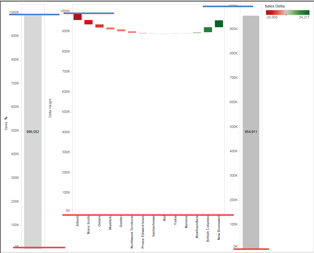
Then, to align height, we use "Reference Line"
In all the case, we need to pick "highest point across three worksheets".
Because we sorted Delta as acsending, the highest point is max of last year or this year.
[Sales Last year] // already exist
{fixed:sum(if [Header Time Range] ="Last Year 3 months" then [Sales] else 0 end)}
[Sales This year]
{fixed:sum(if [Header Time Range] ="Curent 3 months" then [Sales] else 0 end)}
[Max Height for Ref Line]
max([Sales Last year],[Sales This year])
Put [Max Height for Ref Line] to Detail shelf and set "Reference Line".
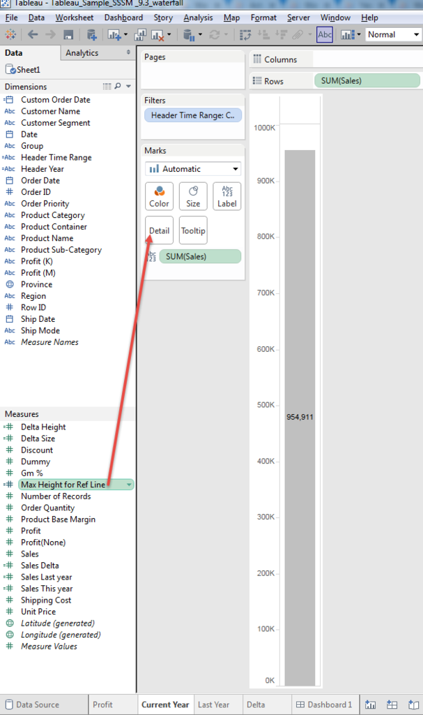
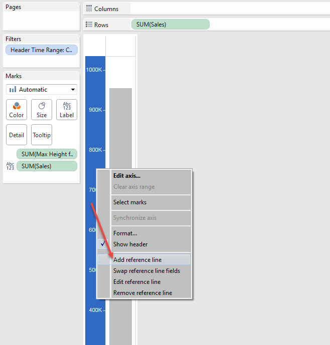
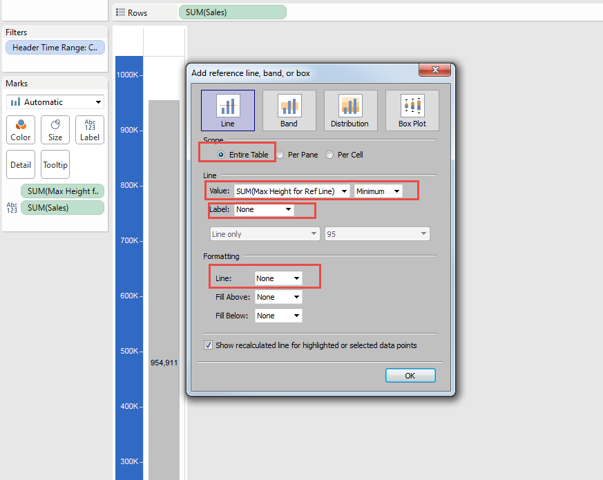
Same thing for other two sheets, and let's see dashboard.
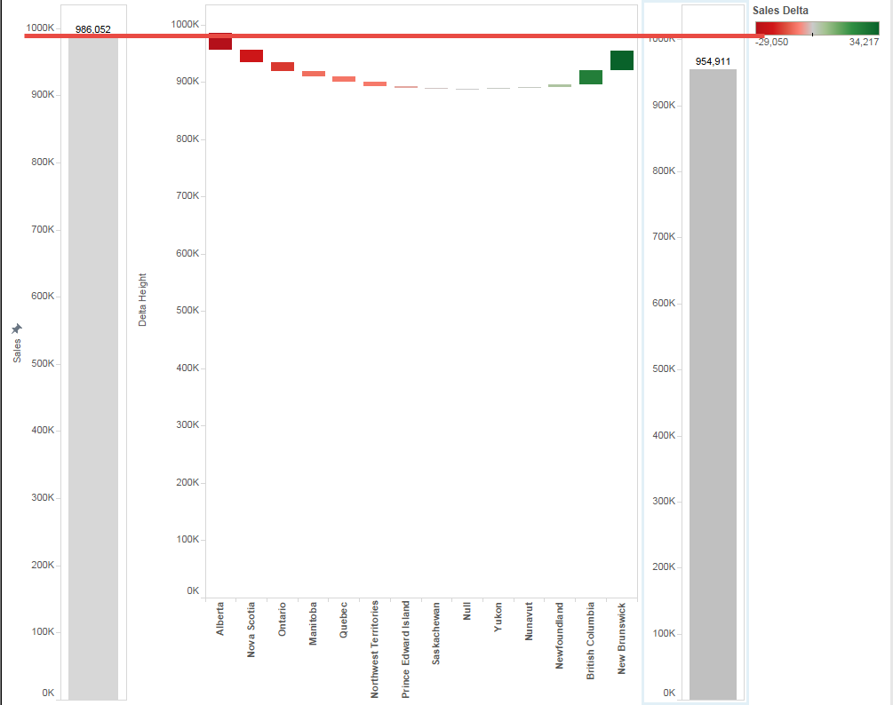
It's still miss-alighed.
Because of "Text" on top of the bar chart.
We still want to keep the text, so change the positoin.
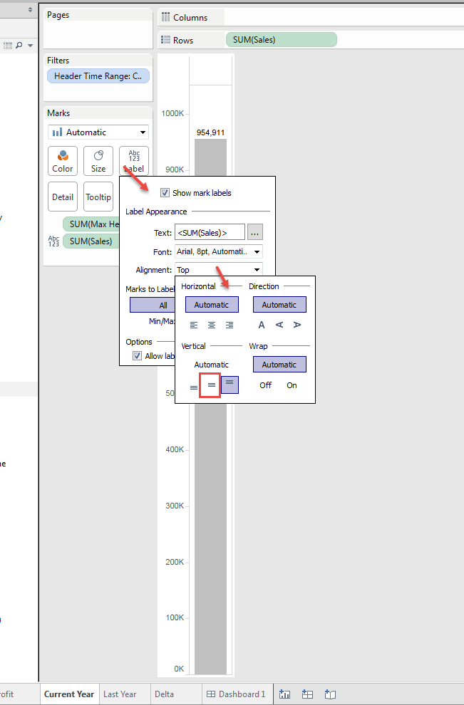
Let's see the dashboard again.
Now last year and Current year is aligned, but Delta still little bit off.
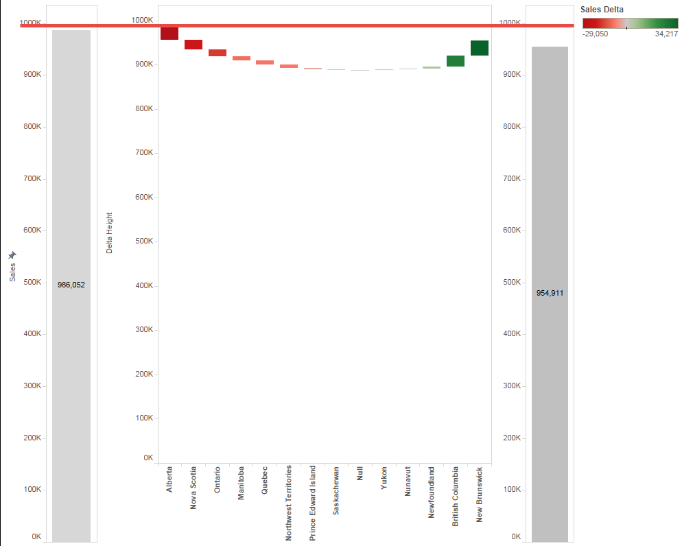
We need to align Zero Line to fix this.
We can add "Blank" box on Dashboard, but I'm afraid it changes the size according to the screen size.
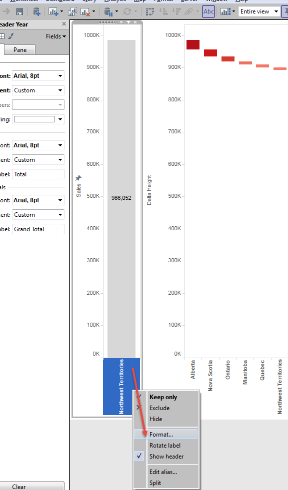
To algen Zero line, we need to add dummy header.
Let's fix Wrap or Not because it changes the Zero line position under "Automatic setting"
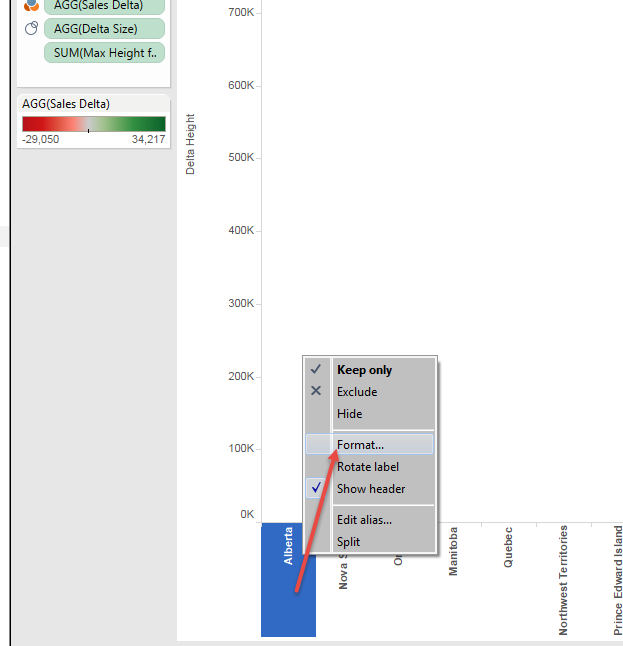
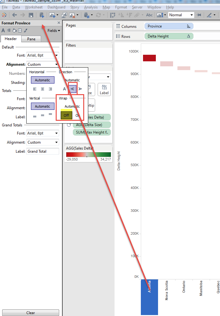
Then we add Header to Last year and Current year worksheets.
To align the height of header, we want to pick longest Province name
[Header Year]
{fixed:max(if len([Province])={fixed:max(len([Province]))} then [Province] end)}
Then put this field to both sheets.

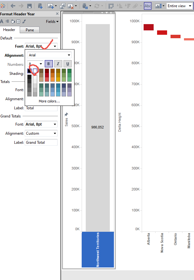
Then Change the Font color of Dummy Header to white.
You can add "text" tile with floating.
(This is off-position little bit when the screen size changes)

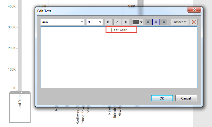
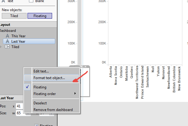
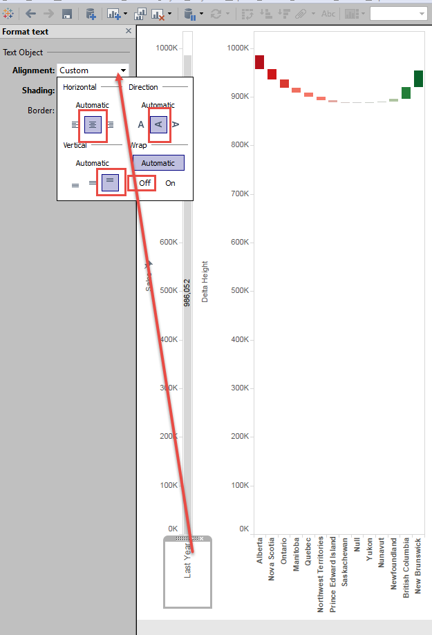
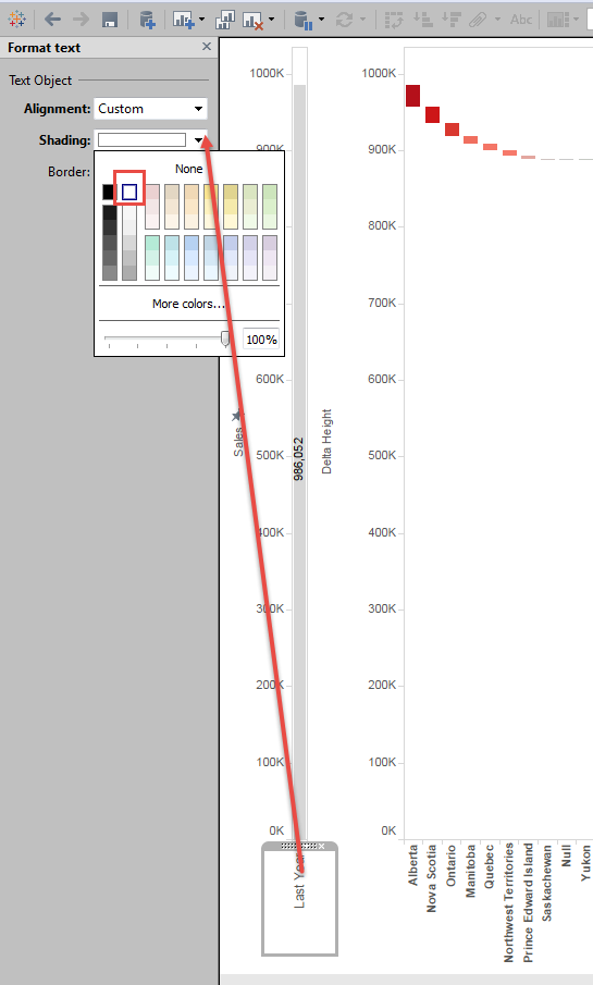
Same thing for Current Year.
Then Hide Header from both Delta and Currenmt Year.
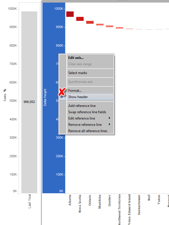
Finally you got completed water fall chart.
Enjoy Tableau!